Learning to read from memory with a neural network

To compute complex functions, computers rely on the ability to read from and write to memory. This ability is missing, however, from standard deep neural neural networks (DNNs), and research has shown that reading and writing to external memory facilitates certain types of computation. But how can we train a DNN to access memory? Both reading and writing are non-differentiable functions—as devised in digital computers—so they are incompatible with backpropagation which is the standard approach to training a DNN. There has been a substantial amount of work that infuses recurrent neural networks with external memory; however, in this post, we’ll make use of the Gumbel-softmax reparameterization to allow a feedforward DNN to read from an external memory bank.

Integers and indexing

A real-world digital computer has a finite bank of memory which is addressed with a binary number. When written to, the memory location associated with that number stores a value that the computer can load for later processing. This ability to store and load data to memory enables computers to compute a large class of functions (that is, the set of functions that are computable by a Turing machine or any equivalent model of computation). Theoretically, recurrent neural networks are capable of simulating a Turing machine and, consequently, can compute the same set of functions. However, to the best of my knowledge, no such proof has been shown for feedforward networks (especially ones of finite-depth and width).

Let's briefly consider how memory works in a real-world computer. Suppose you have a computer with 16-bit memory. You might have an instruction located at memory address (hexadecimal) 0x0000 and a datum, necessary for some computation, stored at 0x1000. Suppose the computer has an instruction at 0x0000 saying to load the datum at 0x1000 to a register. When the computer is started—in this simplistic example—a piece of circuitry called a program counter will configure the state of the circuitry in the CPU to load the instruction at 0x0000 which configure the state of the circuitry to load the datum at 0x1000 into a specified register and used for the further computation (that is, the instructions that follow 0x0000).

Standard feedforward DNNs cannot learn to do this type of loading or any type of loading similar to this from an external memory source. DNNs have real-valued (really, floating-point) parameters and treat input and output as real-valued arrays of numbers, even if the input and output are integer-valued (or, as in the case of categorical variables, can be mapped to the integers). For example, 2D natural images are often composed of integers between 0 and 255; however, this property is ignored in standard DNNs and all inputs are cast to real numbers. In classification tasks, the output of the network—before any user-defined thresholding or argmax operation—represents a probability and is correspondingly real-valued. This transformation from integers to real-valued numbers is necessary for backpropagation to update the weights of the DNN.

But what if you are in a situation where you require integer-values in the middle of the network? A naive solution would be to use rounding. This, however, is non-differentiable (or at least has a zero gradient almost everywhere). So if rounding is used, the DNN cannot update its weights.

Let’s assume that we are working with an external memory bank that is an array of numbers (a tensor, if you like), and the job of the network is to calculate the (one-hot) index location of a value in that memory bank. An way to do this is to allow for some fuzziness and take a weighted average of several locations (using the softmax function on what represents the memory indices) as in the Neural Turning Machine. However, I’d argue that soft indexing is not as interpretable as simply addressing one location from memory.

As a silly example to illustrate the point, let’s say you want to train one end-to-end DNN to compare user-input pictures of dogs and cats to a prototypical picture of a dog and cat based on whatever class of image the user input (e.g., compare a user-input picture of a cat, in some way, to the prototypical picture of a cat). If you use soft indexing, then the input to the comparison section of the network will be comparing a pixelwise weighted average of the prototypical cat and dog image to the user image. The more desirable function of the DNN would be to use only the prototypical cat image if the user image is of a cat and likewise for a dog.

Hard indexing with the Gumbel-softmax reparameterization

We can create hard indices—true one-hot index vectors—through a trick called the Gumbel-softmax (GS) reparameterization. The GS relaxes the hard indexing into a soft indexing problem that can be (asymptotically) viewed as an argmax operation.

Similar to the Gaussian reparameterization discussed in the variational autoencoder, the GS allows backpropagation to work with a sampling step in the middle of a DNN—a normally non-differentiable operation. GS works by changing the sampling operation in such a way that all of the component operations are differentiable. While there are other ways that you can estimate the gradient of a function of integer-valued variables, the GS reparameterization provides a better estimate of the gradient (in the sense that the gradient estimate has lower variance).

While the theoretical construction of the GS is outside the scope of this post, I'll give a high-level overview of how the GS works and provide working code in PyTorch. Suppose we have a neural network $f(\cdot)$ with a hidden layer $f_i(\cdot)$ producing a representation $h \in \mathbb{R}^n$ that we intend to use as memory indices.

To use $h$ to create a one-hot vector that indexes a memory location we:

1. Generate a sample $g\in\mathbb{R}^n$ from a Gumbel distribution,
2. Add $h$ and $g$,
3. Divide the result by a temperature value $\tau > 0$,
4. Take softmax of the result.

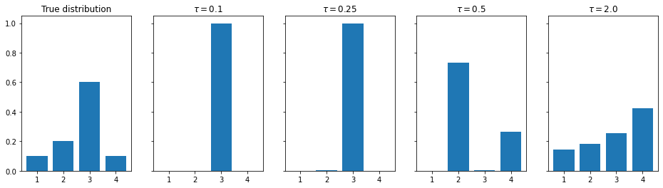
The temperature value $\tau$, as it goes to zero, makes the softmax operation functionally equivalent to an argmax operation. An example of the result is shown in Fig. 1 where an example distribution is given in the left-most image and the result of the GS sampling process is given in the four plots to the right, each with different values of $\tau$. We see that, as $\tau$ gets close to 0, the sampling does function as an approximate argmax operation. When $\tau$ grows, the less the operation looks like an argmax. In practice, setting $\tau$ very close to zero causes exploding gradients which make training unstable, so we set $\tau$ reasonably low or scale it down it as training progresses.

Because we cannot set $\tau$ to zero, we will have non-zero values in other indices—a result that we want to avoid according to the problem setup. We will use the straight-through GS trick to create a true one-hot vector. Let $y$ be the output of the GS and let $y_{\mathrm{oh}}$ be the one-hot construction of the argmax of $y$. Then the straight-through GS simply does the following:

$$ y_{\mathrm{st}} = \mathrm{detach}(y_{\mathrm{oh}} - y) + y,$$

where $\mathrm{detach}(\cdot)$ detaches the argument from the computation graph keeping track of the gradients for backpropagation. Adding a number is differentiable and the resulting number, $y_{\mathrm{st}}$ has the same values as $y_{\mathrm{oh}}$ but is still on the computation graph (with the gradients of $y$).

Implementing the above in PyTorch is simple and the code is below where the gumbel_softmax function takes in the hidden representation (e.g., $h$) and outputs the straight-through GS result.

def sample_gumbel(logits, eps=1e-8):
    U = torch.rand_like(logits)
    return -torch.log(-torch.log(U + eps) + eps)

def sample_gumbel_softmax(logits, temperature):
    y = logits + sample_gumbel(logits)
    return F.softmax(y / temperature, dim=-1)

def gumbel_softmax(logits, temperature=0.67):
    y = sample_gumbel_softmax(logits, temperature)
    shape = y.size()
    _, ind = y.max(dim=-1)
    y_hard = torch.zeros_like(y).view(-1, shape[-1])
    y_hard.scatter_(1, ind.view(-1, 1), 1)
    y_hard = y_hard.view(*shape)
    return (y_hard - y).detach() + y

Learning to address memory

I’ll show a very basic example of a network that can learn to address a memory location using the Gumbel-softmax. (A Jupyter notebook with the full implementation can be found here.)

We’ll have a feedforward neural network fit a (noisy) quadratic function using a memory bank of 5 values uniformly spaced in the interval $[0, 1]$. If the network learns to pick the correct values of the memory bank, we should see the resulting estimator get close to the best piecewise constant estimate of the true quadratic function, where the constants are those values in the memory bank.

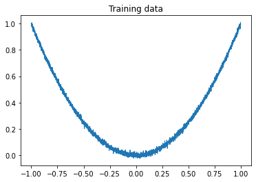
The training data—shown in Fig. 2—will consist of values between -1 and 1, representing the independent variable $x$, with corresponding dependent variables $y=x^2+\varepsilon$ where $\varepsilon \stackrel{iid}{\sim} \mathcal N(0,\sigma^2)$.

The network will consist of a few fully-connected layers using batch norm and ReLU activations (but no ReLU or batch norm on the final layer).

The output of these several layers will be fed into the gumbel_softmax function, as described in the previous section, and the resulting one-hot vector will be used to address the memory bank by simply matrix multiplying (or taking the inner product, if you prefer) the one-hot vector with the memory bank. An example implementation of external memory for our simple setup is shown in PyTorch below, where the the instantiation argument is a tensor $\mathrm{memory} \in \mathbb{R}^m$ and $\mathrm{idx} \in \mathbb{R}^{n\times m}$ where $m$ is the number of memory elements and $n$ is the batch size.

class MemoryTensor(nn.Module):
    def __init__(self, memory:Tensor):
        super().__init__()
        memory.unsqueeze_(1)
        self.memory = memory
        
    def __getitem__(self, idx:Tensor):
        if self.training:
            idx = gumbel_softmax(idx)
            out = idx @ self.memory
        else:
            idx = torch.argmax(idx, dim=1)
            out = self.memory[idx]
        return out

The MemoryTensor can then be indexed in the network with something like the following (where net is some neural network that outputs a tensor $\mathbb{R}^{n\times 3}$ in this illustration which is not specifically related to the experiment).

memory = MemoryTensor(torch.tensor([1.,2.,3.]))
idx = net(x)
y = memory[idx]

Note that when training the MemoryTensor uses the GS, and when in production it uses argmax. The argmax is often more appropriate in production because it removes the random sampling; in some cases, the random sampling may be desired but not in this application.

Because only one location of the memory bank is 1 and all other entries are 0 (in both training and production), the result will consist only of the value from one memory location; that is, the network will have functionally addressed a memory location and read its value.

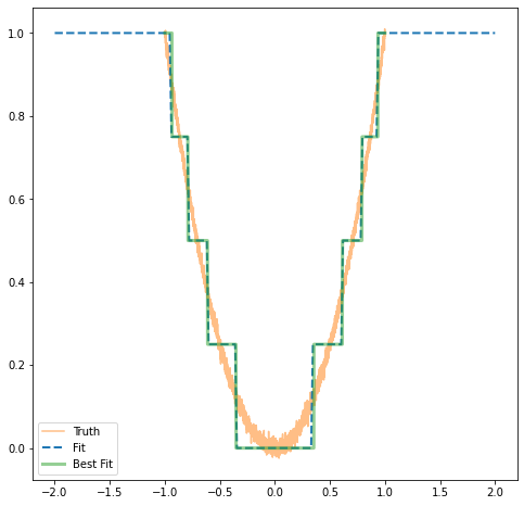
We train the network for several hundred iterations with the Adam optimizer using MSE as a loss function and get the result seen in Fig. 3 in the dashed blue "Fit" line. The optimal fit—the best piecewise constant estimate of the quadratic—using the values in memory is shown in the solid green line labeled "Best Fit." The two are (qualitatively) nearly identical and we can say that this simple experiment was successful.

Caveat: This method will not know how to use additional memory locations. If you doubled the resolution of the memory bank, the network would fail to use that extra information. So this form of memory addressing is brittle. But, you could swap the memory out for another set of variables if the mapping was the same. For example, if the quadratic was changed to $2x^2$, then you could swap the memory with the values multiplied by two and expect the same performance. Something you can’t do with a standard neural network.

Takeaways

We showed a method to read from external memory inside a feedforward neural network, which is normally an operation that prevents the network from being trained. We used the Gumbel-softmax reparameterization to create true one-hot vectors that index one location in memory, and we walked through a toy experiment showing that the proposed method to read from memory does work as expected.

While the toy experiment was too simplistic to showcase the possibilities of this framework, you can, for example, easily extend this method train a network to read from a bank of images. Like the cat and dog example discussed in the Integers and Indexing section, it seems plausible that there are scenarios where you want to use some prototypical or ideal examples of a class of images inside the network to be used for further processing or improve the performance on some task. To be more concrete, training a network end-to-end with an external memory bank of images could be used to improve classification (e.g., find a nearest example) or improve multi-atlas segmentation by choosing the best image to register to another image.

Regardless of whether you believe that this method can improve performance in the concrete examples above, the research points to the fact that reading from external memory does facilitate certain types of computation, and this method is one simple way to do so—potentially increasing the space of functions practically approximated by a feedforward neural network.