Aleatory or epistemic? WTF are those?

Deep neural networks (DNNs) are easy-to-implement, versatile machine learning models that can achieve state-of-the-art performance in many domains (for example, computer vision, natural language processing, speech recognition, recommendation systems). DNNs, however, are not perfect. You can read any number of articles, blog posts, and books discussing the various problems with supervised deep learning. In this article we'll focus on a (relatively) narrow but major issue: the inability for a standard DNN to reliably show when it is uncertain about a prediction. For a Rumsfeldian take on it: The inability of DNNs to know "known unknowns."

As a simple example of this failure mode in DNNs, consider training a DNN for a binary classification task. You might reasonably presume that the softmax (or sigmoid) output of a DNN could be used to measure how certain or uncertain the DNN is in its prediction; you would expect that seeing a softmax output close to 0 or 1 would indicate certainty, and an output close to 0.5 would indicate uncertainty. In reality, the softmax outputs are rarely close to 0.5 and are, more frequently than not, close to 0 or 1 regardless of whether the DNN is making a correct prediction. Unfortunately, this fact makes naive uncertainty estimates unreliable (for instance, entropy over the softmax outputs).

To be fair, uncertainty estimates are not needed for every application of a DNN. If a social media company uses a DNN to detect faces in images so that its users can more easily tag their friends, and the DNN fails, then the failure of the method is nearly inconsequential. A user might be slightly inconvenienced, but in low-stakes environments like social media or advertising, uncertainty estimates aren't vital to creating value from a DNN.

In high-stakes environments, however, like self-driving cars, health care, or military applications, a measure of how uncertain the DNN is in its prediction could be vital. Uncertainty measurements can reduce the risk of deploying a model because they can alert a user to the fact that a scenario is either inherently difficult to do prediction in, or the scenario has not been seen by the model before.

In a self-driving car, it seems plausible that a DNN should be more uncertain about predictions at night (at least in the measurements coming from optical cameras) because of the lower signal-to-noise ratio. In health care, a DNN that diagnoses skin cancer should be more uncertain if it were shown a particularly blurry image, especially if the model had not seen such blurry examples in the training set. In a model to segment satellite imagery, a DNN should be more uncertain if an adversary changed how they disguise certain military installations. If the uncertainty inherent in these situations were relayed to the user, the information could be used to change the behavior of the system in a safer way.

In this article, we explore how to estimate two types of statistical uncertainty alongside a prediction in a DNN. We first discuss the definition of both types of uncertainty, and then we highlight one popular and easy-to-implement technique to estimate these types of uncertainty. Finally, we show and implement some examples for both classification and regression that makes use of these uncertainty estimates.

For those who are most interested in looking at code examples, here are two Jupyter Notebooks one with a toy regression example and the other with a toy classification example. There are also PyTorch-based code snippets in the "Examples and Applications" section below.

What do we mean by 'uncertainty'?

Uncertainty is defined by the Cambridge Dictionary as: "a situation in which something is not known." There are several reasons why something may not be known, and—taking a statistical perspective —we will discuss two types of uncertainty called aleatory (sometimes referred to as aleatoric) and epistemic uncertainty.

Aleatory uncertainty relates to an objective or physical concept of uncertainty—it is a type of uncertainty that is intrinsic to the data-generating process. Since aleatory uncertainty has to do with an intrinsic quality of the data, we presume it cannot be decreased by collecting more data; that is, it is irreducible.

Aleatory uncertainty can be explained best with a simple example: Suppose we have a coin which has some positive probability of being heads or tails. Then, even if the coin is biased, we cannot predict—with certainty—what the next toss will be, regardless of how many observations we make. (For instance, if the coin is biased such that heads turn up with probability 0.9, we might reasonably guess that heads will show up in the next toss, but we cannot be certain that it will happen.)

Epistemic uncertainty relates to a subjective or personal concept of uncertainty—it is a type of uncertainty due to knowledge or ignorance of the true data-generating process. Since this type of uncertainty has to do with knowledge, we presume that it can be decreased (for example, when more data has been collected and used for training); that is, it is reducible.

Epistemic uncertainty can be explained with a regression example. Suppose we are fitting a linear regression model and we have independent variables $x$ between -1 and 1, and corresponding dependent variables $y$ for all $x$. Suppose we chose a linear model because we believe that when $x$ is between -1 and 1, the model is linear. We don't, however, know what happens when a test sample $x'$ is far outside this range; say at $x'$ = 100. So, in this scenario, there is uncertainty about the model specification (for example, the true function may be quadratic) and there is uncertainty because the model hasn't seen data in the range of the test sample. These uncertainties can be bundled into uncertainty regarding the knowledge of true data-generating distribution, which is epistemic uncertainty.

The terms aleatory and epistemic, with regards to probability and uncertainty, seem to have been brought into the modern lexicon by Ian Hacking in his book "The Emergence of Probability," which discusses the history of probability from 1600–1750. The terms are not clear for the uninitiated reader, but their definitions are related to the deepest question in the foundations of probability and statistics: What does probability mean? If you are familiar with terms frequentist and Bayesian, then you will see the respective relationship between aleatory (objective) and epistemic (subjective) uncertainty. I'm not about to solve this philosophical issue in this blog post, but know that the definitions of aleatory and epistemic uncertainty are nuanced, and what falls into which category is debatable. For a more comprehensive (but still applied) review of these terms, take a look at the article: "Aleatory or Epistemic? Does it matter?"

Why is it important to distinguish between aleatory and epistemic uncertainty? Suppose we are developing a self-driving car, and we take a prototype that was trained on normal roads and have it drive through the Monza racing track, which has extremely banked turns.

Since the car hasn't seen the situation before, we would expect the image segmentation DNN in the self-driving car, for example, to be uncertain because it has never seen the sky nearly to the left of ground. In this case, the uncertainty would be classified as epistemic because the DNN doesn't have knowledge of roads like this.

Suppose instead that we take the same self-driving car and take it for a drive on a rainy day; assume that the DNN has been trained on lots of rainy-day conditions. In this situation, there is more uncertainty about objects on the road simply due to lower visibility. In this case, the uncertainty would be classified as aleatory because there is inherently more randomness in the data.

These two situations should be dealt with differently. In the race track, the uncertainty could tell the developers that they need to gather a particular type of training data to make the model more robust, or the uncertainty could tell the car could try to safely maneuver to a location where it can hand-off control to the driver. In the rainy-day situation, the uncertainty could alert the system to simply slow down or enable certain safety features.

Estimating uncertainty in DNNs

There has been a cornucopia of proposed methods to estimate uncertainty in DNNS in recent years. Generally, uncertainty estimation is formulated in the context of Bayesian statistics. In a standard DNN for classification, we are implicitly training a discriminative model where we obtain maximum-likelihood estimates of the neural network weights (depending on the loss function chosen to train the network). This point-estimate of the network weights is not amenable to understanding what the model knows and does not know. If we instead find a distribution over the weights, as opposed to the point-estimate, we can sample network weights with which we can compute corresponding outputs.

Intuitively, this sampling of network weights is like creating an ensemble of networks to do the task: We sample a set of "experts" to make a prediction. If the experts are inconsistent, there is high epistemic uncertainty. If the experts think it is too difficult to make an accurate prediction, there is high aleatory uncertainty.

In this article, we'll take a look at a popular and easy-to-implement method to estimate uncertainty in DNNs by Yarin Gal and Zoubin Ghahramani. They showed that dropout can be used to learn an approximate distribution over the weights of a DNN (as previously discussed). Then, during prediction, dropout is used to sample weights from this fitted approximate distribution—akin to creating the ensemble of experts.

Epistemic uncertainty is estimated by taking the sample variance of the predictions from the sampled weights. The intuition behind relating sample variance to epistemic uncertainty is that the sample variance will be low when the model predicts nearly identical outputs, and it will be high when the model makes inconsistent predictions; this is akin to when the set of experts consistently makes a prediction and when they do not, respectively.

Simultaneously, aleatory uncertainty is estimated by modifying a DNN to have a second output, as well as using a modified loss function. Aleatory uncertainty will correspond to the estimated variance of the output. This predicted variance has to do with an intrinsic quantity of the data, which is why it is related to aleatory uncertainty; this is akin to when the set of experts judges the situation too difficult to make a prediction.

Altogether the final network structure is something like what is shown in Fig. 2. There is an input x which is fed to a DNN with dropout after every layer (dropout after every layer is what is originally specified, but—in practice—dropout after every layer often makes training too difficult). The output of this DNN is an estimated target $\hat{\mathbf{y}}$ and an estimated variance or scale parameter $\hat{\sigma}^2$.

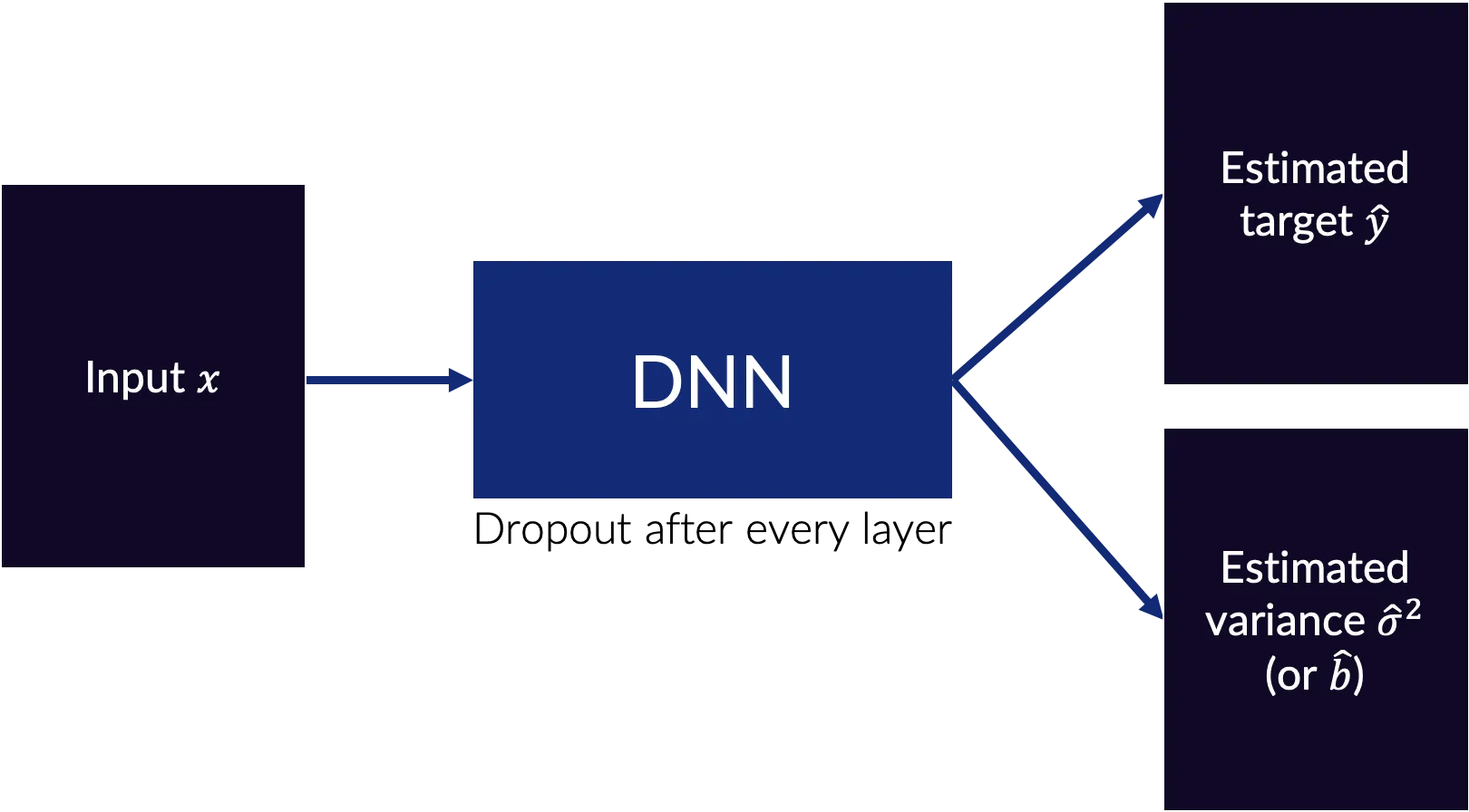
This DNN is trained with a loss function like:

$$ \mathcal{L}(\mathbf{y}, (\hat{\mathbf{y}},\hat{\sigma}^2)) = \frac{1}{M} \sum_{i=1}^M \frac{1}{2} \hat{{\sigma}}_i^{-2} \lVert \mathbf{y}_i - \mathbf{\hat{y}}_i \rVert_2^2 + \frac{1}{2} \log \hat{\sigma}_i^2 $$

or

$$ \mathcal{L}(\mathbf{y}, (\hat{\mathbf{y}}, \hat{\mathbf{b}})) = \frac{1}{M} \sum_{i=1}^M \hat{\mathbf{b}}_i^{-1} \lVert \mathbf{y}_i - \hat{\mathbf{y}}_i \rVert_1 + \log \hat{\mathbf{b}}_i $$

If the network is being trained for a regression task. The first loss function shown above is an MSE variant with uncertainty, whereas the second is an L1 variant. These are derived from assuming a Gaussian and Laplace distribution for the likelihood, respectively, where each component is independent and the variance (or scale parameter) is estimated and fitted by the network.

As mentioned above, these loss functions have mathematical derivations, but we can intuit why this variance parameter captures a type of uncertainty: The variance parameter provides a trade-off between the variance and the MSE or L1 loss term. If the DNN can easily estimate the true value of the target (that is, get ŷ close to the true y), then the DNN should estimate a low variance term on that so as to minimize the loss. If, however, the DNN cannot estimate the true value of the target (for example, there is low signal-to-noise ratio), then the network can minimize the loss by estimating a high variance. This will reduce the MSE or L1 loss term because that term will be divided by the variance; however, the network should not always do this because of the log variance term which penalizes high variance estimates.

If the network is being trained for a classification (or segmentation) task, the loss would look something like this two-part loss function:

$$ \hat{\mathbf{x}}_t = \hat{\mathbf{y}} + \varepsilon_t \qquad \varepsilon_t \sim \mathcal{N}(\mathbf{0},\mathrm{diag}(\hat{\sigma}^2)) $$

$$ \mathcal{L}(\mathbf{x}, \hat{\mathbf{x}}) = \frac{1}{T} \sum_{t=1}^T \mathrm{Cross\ entropy}(\mathbf{x}, \hat{\mathbf{x}}_t) $$

The intuition here with this loss function is: When the DNN can easily estimate the right class of a component, the value $\hat{\mathbf{y}}$ will be high for that class and the DNN should estimate a low variance so as to minimize the added noise (so that all samples will be concentrated around the correct class). If, however, the DNN cannot easily estimate the class of the component, the $\hat{\mathbf{y}}$ value should be low and adding noise can increase the guess, by chance, for the correct class which can overall minimize the loss function. (See Pg. 41 of Alex Kendall's thesis for more discussion on this loss function.)

Finally, in testing, the network is sampled T times to create T estimated targets and T estimated variance outputs. These T outputs are then combined in various ways to make the final estimated target and uncertainty estimates as shown in Fig. 3.

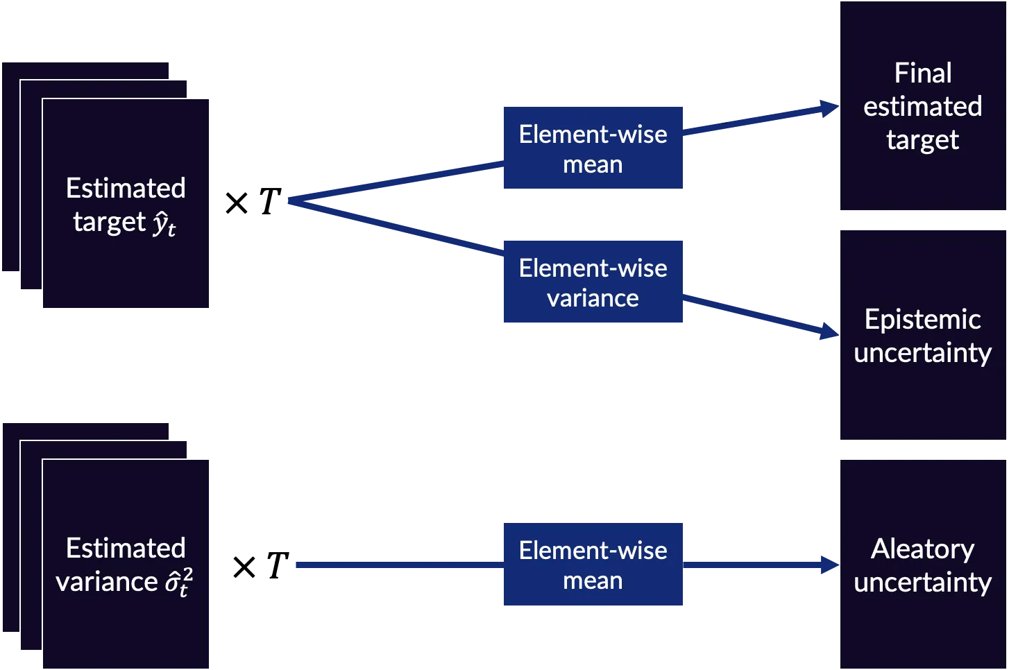
Mathematically, the epistemic and aleatory uncertainty are (for the MSE regression variant):

$$ \mathrm{Aleatory\ uncertainty} = \frac{1}{T} \sum_{t=1}^T \hat{\sigma}^2_t$$

$$ \mathrm{Epistemic\ uncertainty} = \frac{1}{T} \sum_{t=1}^T (\mathbf{\hat{y}}_t - \bar{\mathbf{y}})^2 $$

There are various interpretations of epistemic uncertainty for the classification case: entropy, sample variance, mutual information. Each has been shown to be useful in its own right, and the choice of what type to choose will be application dependent.

Examples and applications

To make the theory more concrete, we'll go through two toy examples for estimating uncertainty with DNNs in a regression and classification task with PyTorch. The code below are excerpts from full implementations which are available in Jupyter notebooks (mentioned at the beginning of the next two subsections). Finally, we'll discuss calculating uncertainty in a real-world data example with medical images.

Regression example

In the regression notebook, we fit a very simple neural network—consisting of two fully-connected layers with dropout on the hidden layer—to one-dimensional input and output data with the MSE variant of the uncertainty loss (implemented below).

class ExtendedMSELoss(nn.Module):
    """ modified MSE loss for variance fitting """
    def forward(self, out:torch.Tensor, y:torch.Tensor) -> torch.Tensor:
        yhat, s = out
        loss = torch.mean(0.5 * (torch.exp(-s) * F.mse_loss(yhat, y, reduction='none') + s))
        return loss

Note that instead of fitting the variance term directly, we fit the log of the variance term for numerical stability.

In the regression scenario, we could also use the L1 variant of the uncertainty loss which is in the notebook and implemented below.

class ExtendedL1Loss(nn.Module):
    """ modified L1 loss for scale param. fitting """
    def forward(self, out:torch.Tensor, y:torch.Tensor) -> torch.Tensor:
        yhat, s = out
        loss = torch.mean((torch.exp(-s) * F.l1_loss(yhat, y, reduction='none')) + s)
        return loss

Sometimes using L1 loss instead of MSE loss results in better performance for regression tasks, although this is application dependent.

The aleatory and epistemic uncertainty estimates in this scenario are then computed as in the implementation below (see the notebook for more context).

def regression_uncertainty(yhat:torch.Tensor, s:torch.Tensor, mse:bool=True) -> Tuple[torch.Tensor, torch.Tensor]:
    """ calculate epistemic and aleatory uncertainty quantities based on whether MSE or L1 loss used """
    # variance over samples (dim=0), mean over channels (dim=1, after reduction by variance calculation)
    epistemic = torch.mean(yhat.var(dim=0, unbiased=True), dim=1, keepdim=True)
    aleatory = torch.mean(torch.exp(s), dim=0) if mse else torch.mean(2*torch.exp(s)**2, dim=0)
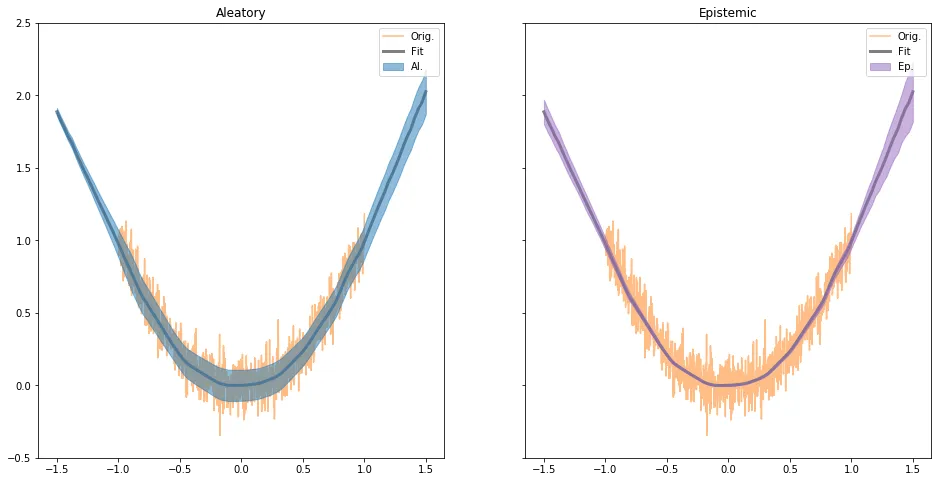
    return epistemic, aleatory

In Fig. 4, we visualize the fit function and the uncertainty results. In the plot to the far right, we show the thresholded epistemic uncertainty which demonstrates the capabilities of uncertainty estimates to detect out-of-distribution data (at least in this toy scenario).

Classification example

In the classification notebook, we, again, fit a neural network composed of two fully-connected layers with dropout on the hidden layer. In this case, we are trying to do binary classification. Consequently, the loss function is as implemented below.

class ExtendedBCELoss(nn.Module):
    """ modified BCE loss for variance fitting """
    def forward(self, out:torch.Tensor, y:torch.Tensor, n_samp:int=10) -> torch.Tensor:
        logit, sigma = out
        dist = torch.distributions.Normal(logit, torch.exp(sigma))
        mc_logs = dist.rsample((n_samp,))
        loss = 0.
        for mc_log in mc_logs:
            loss += F.binary_cross_entropy_with_logits(mc_log, y)
        loss /= n_samp
        return loss

There are numerous uncertainty estimates we could compute in this scenario. In the below implementation, we calculate epistemic, entropy, and aleatory uncertainty. Entropy could reasonably be argued to belong to one of aleatory and epistemic uncertainty, but below it is separated out so that aleatory and epistemic uncertainty are calculated as previously described.

def classification_uncertainty(logits:torch.Tensor, sigmas:torch.Tensor, eps:float=1e-6) -> Tuple[torch.Tensor, torch.Tensor]:
    """ calculate epistemic, entropy, and aleatory uncertainty quantities """
    probits = torch.sigmoid(logits)
    epistemic = probits.var(dim=0, unbiased=True)
    probit = probits.mean(dim=0)
    entropy = -1 * (probit * (probit + eps).log2() + ((1 - probit) * (1 - probit + eps).log2()))
    aleatory = torch.exp(sigmas).mean(dim=0)
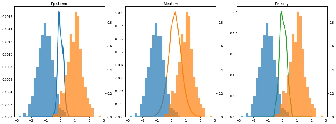
    return epistemic, entropy, aleatory

In Fig. 5, we visualize the resulting epistemic and aleatory uncertainty, as well as entropy, over the training data. As we can see the training data classes overlaps near zero, and the uncertainty measures peak there. In this toy example, all three measures of uncertainty are highly correlated. Discussion as to why is provided in the notebook for the interested reader.

Medical image example

In this last example, I'll show some results and applications of uncertainty in a real-world example published as a conference paper (pre-print here). The task explored is an image-to-image translation task, akin to the notable pix2pix example, but with medical images. In this case, we wanted to make a computed tomography (CT) image of the brain look like the corresponding magnetic resonance (MR) image of the brain. This is a regression loss and we used the MSE variant of the uncertainty loss to train a U-Net modified to have spatial dropout (see here for a discussion as to why spatial dropout) after every layer, and to output two images instead of only one; one output is the estimated MR image and the other is the pixel-wise variance.

Example inputs and outputs are shown in Fig. 6. The CT image on the far left has an anomaly in the left hemisphere of the occipital lobe (lower-left of the brain in the image; it is more easily visualized in the corresponding MR image to the right). The DNN was only trained on healthy images, so the DNN should be ignorant of such anomalous data, and it should reflect this—according to the theory of epistemic uncertainty as previously discussed—by having high sample variance (that is, high epistemic uncertainty) in that region.

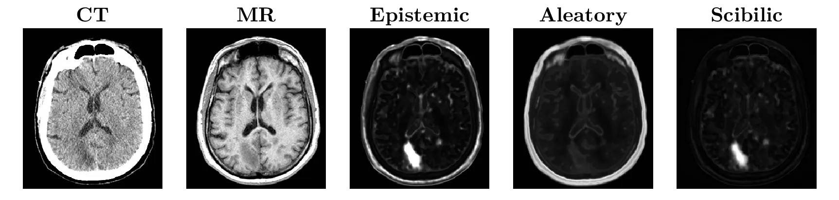
When this image was input to the network, we calculated the epistemic and aleatory uncertainty. The anomaly is clearly highlighted in the epistemic uncertainty, but there are many other regions which are also predicted to have high epistemic uncertainty. If we take the pixel-wise ratio of epistemic and aleatory uncertainty, we get the image shown on the far-right, labeled "Scibilic" (which is discussed more in the pre-print). This image is easily thresholded to predict the anomaly (the out-of-distribution region of the image).

This method of anomaly detection is by no means foolproof. It is quite fickle actually, but it shows a way to apply this type of uncertainty estimation for real-world data.

Takeaways

Uncertainty estimates in machine learning have the potential to reduce the risk of deploying models in high-stakes scenarios. Aleatory and epistemic uncertainty estimates can show the user or developer different information about the performance of a DNN and can be used to modify the system for better safety. We discussed and implemented one approach to uncertainty estimation with dropout. The approach is not perfect, dropout-based uncertainty provides a way to get some—often reasonable—measure of uncertainty. Whether the measure is trustworthy enough to be used in deployment is another matter. The question practitioners should ask themselves when implementing this method is whether the resulting model with uncertainty estimates is more useful—for example, safer—than a model without uncertainty estimates.